MDMx, for Multi-dimensional Mortality, builds model life tables, life table fitting, the prediction of mortality schedules from summary indicators, and mortality forecasting on one decomposition of the Human Mortality Database (HMD). Mortality is treated as a single four-dimensional array, indexed by sex, single year of age, population and calendar year, and a Tucker tensor decomposition of it gives sex and age bases that every population and year share. Each observed mortality schedule of the two sexes then becomes a small matrix of coordinates in one common space, and every tool below works in that space. MDMx is the successor to my SVD-Comp component model of mortality.

Status, November 2026 ▲

MDMx was first written up in two arXiv working papers in March 2026: the framework paper, Multi-dimensional Mortality (MDMx): Sex-Age-Specific Model Life Tables, Fitting, Prediction from Summary Mortality Indicators, and Forecasting, and a companion on forecasting, Mortality Forecasting as a Flow Field in Tucker Decomposition Space. The MDMx app accompanies them.

I am now finishing a thorough revision of the framework paper. It is estimated throughout from the HMD release of 29 October 2026, includes the flow-field forecaster beside MDMx's own, and evaluates both against established forecasting methods from rolling origins. This page describes that revision, from the draft of 9 November 2026. The revised article will be posted together with its code, a single Python package, and a computational companion, a Quarto book that reproduces every figure, table and number in the article.

NB: The results on this page come from a manuscript in preparation, and they can change before it is posted.

The data ▲

Everything is estimated from one release of the HMD, which computes period life tables from official death counts and population estimates with one documented method. Of its 50 populations, 48 are used, from 41 countries and territories. Their series run from 1751 to 2025 but differ widely in length: Sweden's starts in 1751, while only 12 start before 1900. The quantity modelled is the logit of the probability of dying at each single year of age from 0 to 109, for females and males. Of 4,596 curated country-years, 540 are years of war, epidemic or other crisis. They are kept out of the decomposition, and the wars and epidemics are modelled separately.

One basis for every task ▲

The sex and age bases are estimated from the observed schedules alone, with no parametric form in age or in time, and each observed country-year keeps its own coordinates in them. With 50 age components those coordinates represent the observed schedules with a root mean squared error of 0.052 on the logit scale, and their life expectancy differs from the observed by 0.021 years on average. The decomposition is used to obtain the shared basis, not to compress the data. Every schedule the framework generates, fits, predicts or forecasts is a combination of the same age patterns for both sexes, apart from the disruption profile of an exceptional year and the detail that a forecast keeps from the last observed schedule.

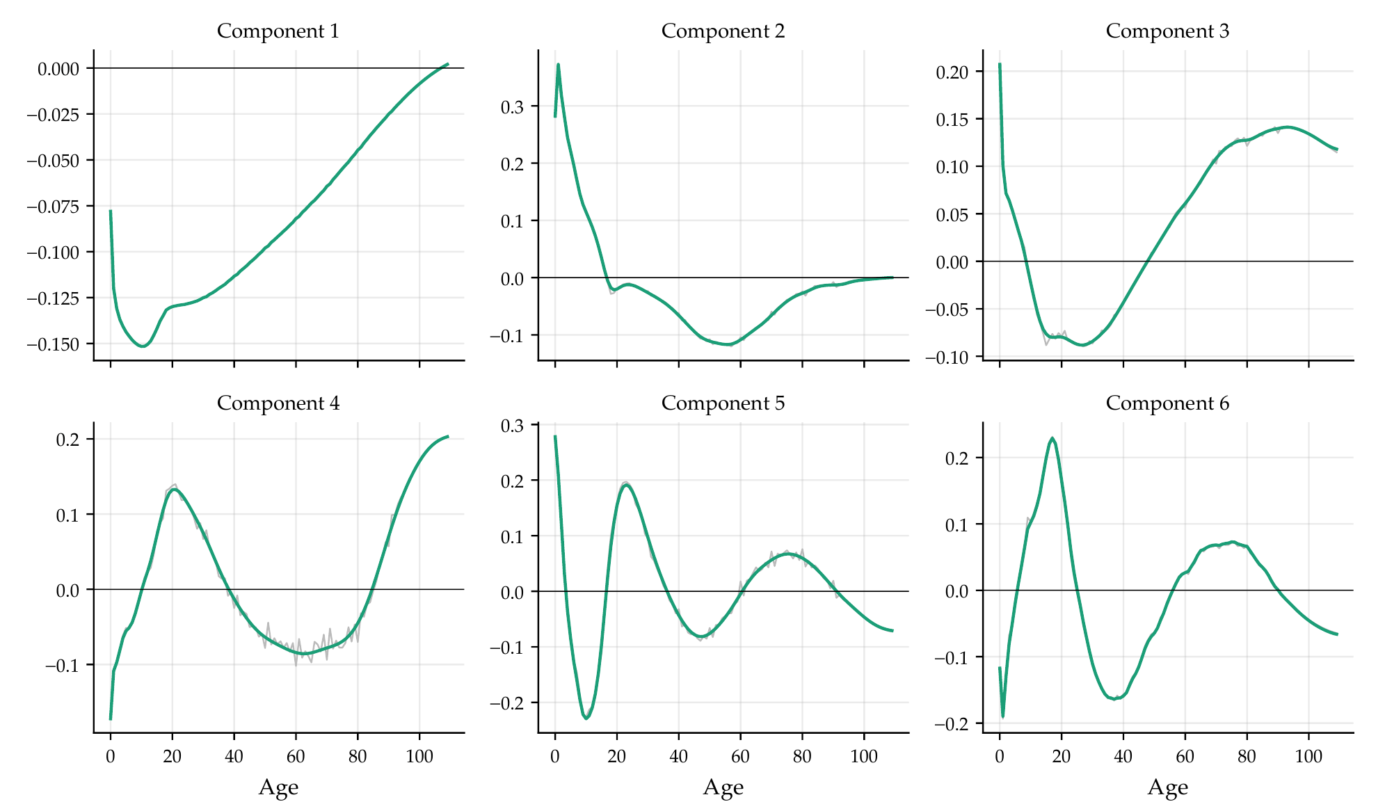Figure 1. The first six of the 50 age basis functions, after smoothing (green) and before (thin grey). The first is close to the mean observed schedule and carries the level of mortality. Each later one changes sign, so it moves mortality between age groups and leaves the level to the first.

Built on the basis:

• A typology of mortality age patterns. Country-years are clustered on how their schedules depart from the schedule that is typical at the same life expectancy. There are five clusters, one of which collects the noisy schedules of small populations. The typology is stable across refits but not when the populations are resampled, so it describes these populations and does not claim types that other populations would reproduce.
• Model life tables at any level of mortality. For a type and a target life expectancy, MDMx generates the schedule of both sexes, calibrated so that its life expectancy is the target exactly.
• Exceptional mortality. A year of war or epidemic is a baseline plus an intensity times a profile over sex and age. One profile per type serves wars and enteric pandemics about as well as one per event; respiratory pandemics differ, because the 1918 influenza struck young adults and COVID-19 the old.
• A life table fitter. Given one life table and nothing else, the fitter estimates its type, its level and whether a disruption is present. On schedules it has not seen, at 5% false positives, it detects 49% of the detectable disruptions, in a median of 2.4 milliseconds. From one schedule alone, a disruption is hard to tell from a change of level.
• Prediction from summary indicators. A neural network predicts the full schedule of both sexes from child mortality (the probability of dying before age 5), or from child and adult mortality (adding the probability of dying between ages 15 and 60), and its predictions reproduce their inputs exactly. This is SVD-Comp rewritten in the Tucker framework; on populations it has not seen, it is as accurate as Log-Quad and SVD-Comp.

Two forecasters ▲

Both forecasters produce the complete schedule of both sexes, at all 110 ages, for every year ahead. They work in the same space, the leading five principal components of the coordinates, and both keep the detail of the population's last observed schedule.

• Anchored MDMx extrapolates each population's own trend, damped and pulled towards the drift of all populations.
• The flow field moves each population along the paths that populations at the same level of mortality followed. Its level moves at the speed observed at that level, pooled over all populations, and, beyond the levels the leading populations have reached, at their recent pace. The rest of the age pattern follows a shape law of the level.

Like bayesLife, the method the United Nations uses to forecast life expectancy, the flow field makes the pace of improvement depend on the level of mortality. Unlike bayesLife, it forecasts the whole schedule of both sexes jointly, with one speed for all populations, estimated without a parametric form.

How the forecasters compare ▲

Twelve entries are compared from forecast origins every five years from 1900 to 2015: anchored MDMx, the flow field, Lee–Carter, the functional model of Hyndman and Ullah, the coherent functional model of Hyndman, Booth and Yasmeen, bayesLife, and an equally weighted ensemble of anchored MDMx, the flow field and Lee–Carter. All but the flow field and the ensemble are fitted both to all years and to the last 50. Each model is fitted only to data for years up to its origin, with a few exceptions that the article lists. The overall comparison ranks the entries on five families of measures (life expectancy of each sex, the gap between the sexes, the sex differences by age, the age pattern, and the prediction intervals) over 20,000 random draws of the families' weights, each with the populations resampled.

The lead is narrower than those shares suggest:

• It depends on the horizon. bayesLife fitted to the last 50 years is first at 1–5 years ahead (86% of the draws) and at 6–10 years (44%, against 35% for the flow field); the flow field is first at 11–15 years (88%).
• On the error of life expectancy alone, the flow field cannot be told apart from the ensemble, nor from Lee–Carter started at the observed rates of the jump-off year, and at 1–5 years ahead the leading methods differ by hundredths of a year.
• Anchored MDMx is in fifth and sixth place of the twelve, and at the shortest horizons it does no better than a random walk with drift.
• From the early origins, 1900–1950, the comparison is contested between the flow field and the ensemble. From the recent origins, 2005–2015, which reach at most 20 years ahead, the flow field is first in 58% of the draws and bayesLife fitted to all years in 42%.
• The flow field's form and MDMx's anchor were selected on origins up to 2010, which favours them.
• At long horizons every structured forecaster under-predicts life expectancy, mainly because old-age mortality fell faster than any of them carried forward.

The research preview, updated on 10 November 2026, summarises the same results. Its 1 November version reports an earlier state of this evaluation; where its numbers differ from those here, these are the later ones.

What the flow field says about mortality change ▲

Fitted to all the data, the flow field implies an annual gain in life expectancy at every level of life expectancy, which can be read against what is known about mortality change. The implied gain rises to 0.44 years a year at a life expectancy of 59 and slows once life expectancy passes about 70. A dip near 71 comes mostly from the stagnation of the 14 populations of Central and Eastern Europe, which a speed pooled over all populations reads as a property of the level. Along the same path the gap between female and male life expectancy widens and then narrows: 3.2 years at a life expectancy of 45, 7.2 years at 70 and 5.3 at 80. The sources of the gains rotate from the young to the old, with ages 0–14 giving 68% of a gain at a life expectancy of 45 and 6% at 80, and ages 65 and over 4% and 58%.

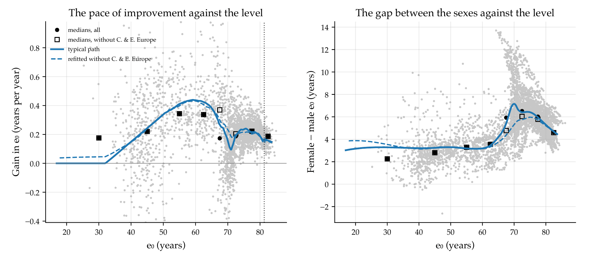Figure 2. What the flow field fitted to all the data implies. Left: the annual gain in life expectancy against its level, observed (grey points; dots are medians, open squares the medians without Central and Eastern Europe) and implied by the flow field (solid line; dashed, refitted without those populations). The dotted vertical line marks the frontier point, beyond which few populations show how mortality improved. Right: female minus male life expectancy against the level, in the same way.

Limits and next steps ▲

The HMD is not globally representative. Its populations are mostly European, with several other high-income countries, and it includes no country of sub-Saharan Africa, South Asia or South-East Asia and little of Latin America. Other data are needed to apply the bases, the typology, the disruption profiles and the forecasters elsewhere, for example where HIV/AIDS has produced age patterns with no analogue in the HMD.

The next step is a second data set, the single-age life tables of the United Nations' World Population Prospects, which cover every country. For the forecasters, most of the remaining error lies in the pace of improvement at old ages and at the frontier. Beyond forecasting, the framework can supply the mortality input of population projections, and the same decomposition can be applied to fertility, so that the components of population change share one framework.

Background ▲

MDMx is the latest step in work that began with my dissertation, where I used the singular value decomposition (SVD) to build a component model of mortality and applied it to the mortality of 19 sites of the INDEPTH Network in Africa and Asia, at a time when no model life table system represented sub-Saharan Africa. A later working paper used model-based clustering to find typical age patterns of mortality in the HMD and built a system of model life tables on them (Clark and Sharrow, 2011). SVD-Comp then predicted complete single-year-of-age schedules from child mortality, or from child and adult mortality; a version of it has been part of the United Nations' World Population Prospects since the 2022 revision.

Those methods work on mortality flattened into a matrix, which gives each sex, or each population, a basis of its own. MDMx keeps sex, age, population and year apart, so that the sex and age bases are shared while each country-year keeps coordinates of its own. An interactive tutorial explains the SVD, SVD-Comp, and how MDMx extends them.

Papers and links ▲

• Multi-dimensional Mortality (MDMx): Sex-Age-Specific Model Life Tables, Fitting, Prediction from Summary Mortality Indicators, and Forecasting, arXiv:2603.20518 (March 2026); the revision described here will update it.
• Mortality Forecasting as a Flow Field in Tucker Decomposition Space, arXiv:2603.24299 (March 2026).
• MDMx app (Shiny), which accompanies the March working papers.
• Flow-field research preview (updated 10 November 2026).
• SVD tutorial: the SVD, SVD-Comp and MDMx.
• SVD-Comp, the component model that MDMx extends.
• Human Mortality Database, the source of the data.